Dimensional Modeling 101: What It Is, Why It Matters, and How It Compares

A practical guide to star schemas, facts, dimensions, and when to use them

In the world of analytics, we have data sources, ETL/ELT processes, and end-analyses or insights. Data modeling comes into play, as part of the “T” of ETL/ELT. And dimensional modeling is one of the methods to transform data in the way that makes downstream analytics and reporting easier and efficient. Dimensional modeling is such a commonly implemented technique for analytics across many industries and companies. As a data practitioner, you won’t get away NOT understanding dimensional modeling if you want to thrive in your data career.

In this article, we’ll cover what dimensional modeling is, how it works, and some of the trade-offs compared to other modeling methods.

1. What is Dimensional Modeling

2. Normalization and Denormalization

3. Facts and Dimensions

4. Dimensional Model Design Process

5. Other Data Modeling Techniques

You’ll see no fluff, just simple explanations and examples of what you need to know in getting started with dimensional modeling. If you’re already familiar with it, then this article will be a good refresher for you.

In this article, we use “data warehouse“ and “data lakehouse” interchangeably.

What is Dimensional Modeling

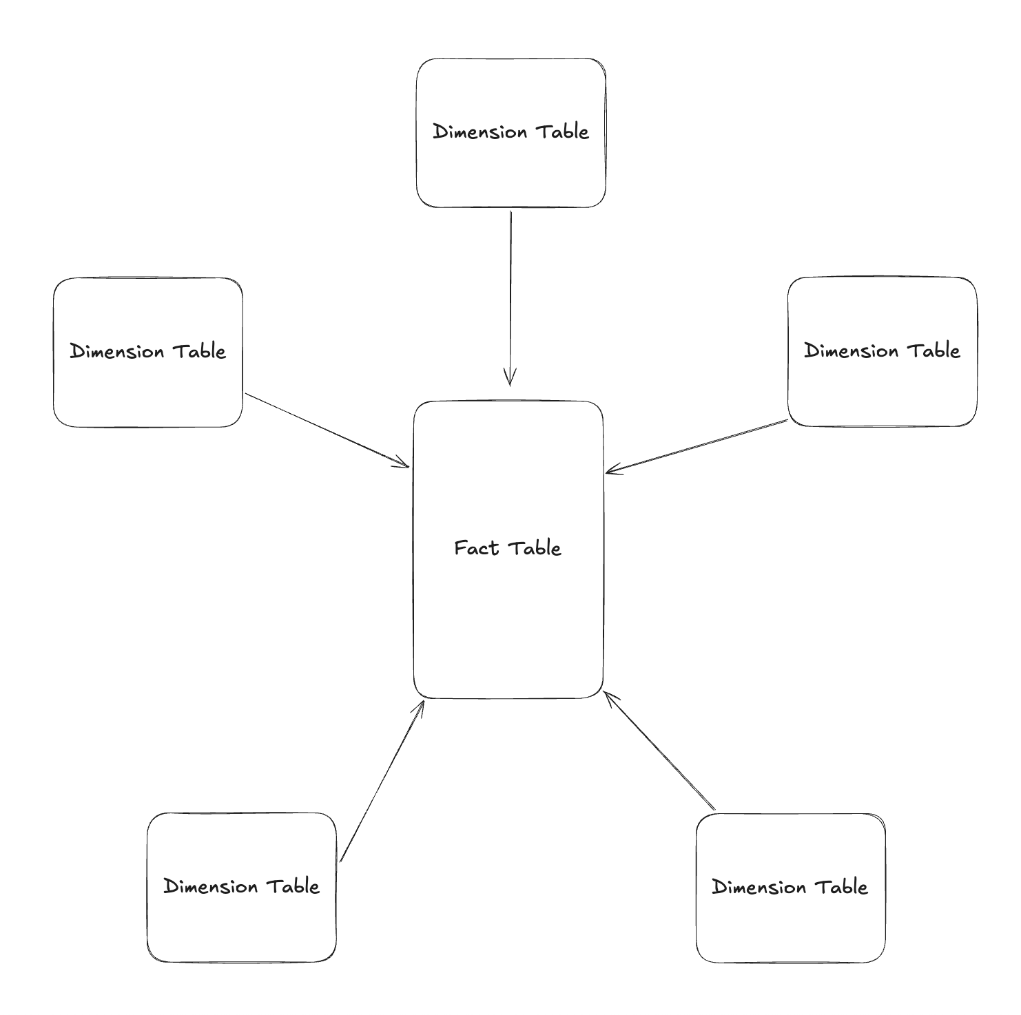
Dimensional modeling is a data modeling method optimal for analytics and reporting use cases. An end-product of dimensional modeling is often called “Star Schema“, as it looks like a star when visualizing the model.

What does it mean when we say “optimal for analytics and reporting“?

It means that dimensional modeling is:

• Efficient for read operations (e.g. “select” in sql)

• Effective in laying out the information in such a way that’s easier for people to understand and use the data for downstream use cases

A core idea in understanding dimensional modeling is database normalization and denormalization. Let’s take a look at both.

Normalization and Denormalization

Normalization

If you think about how data behind a software or an app is structured, what do you image it would look like?

The answer is—They’re highly “normalized”, meaning it’s built in the way that reduces data redundancy. Because many users use the app, data is always getting added and updated concurrently. So, normalized data is optimal for “write”, “update“, and “delete“ operations (e.g. “insert”, “update“, and “delete“ in sql).

For example, let’s say you own a retail store. You have several products with different categories. In an normalized format, the data would look like this:

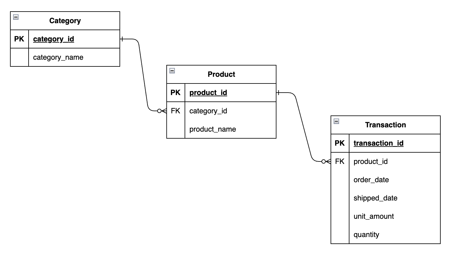
As you can see, fields like product_name and category_name are in its own entity/table (Product and Category). This means that when you need to make a change, like adding a new product or updating an existing product, you can do it in one place. Product and category names are NOT duplicated across other tables, each value appears only once in one table.

And less data duplication gives you some benefits such as:

• Data Integrity

• Consistency

• Maintenance Efficiency

We can talk about the level of normalization, but we won’t go into it in this article. The least thing I’d tell you is that 3rd normal form is the standard in normalized databases. From a high level view, the less data duplication you see, the more normalized your data structure is.

And that’s what database normalization is in essence, and why many operational databases (OLTP, databases behind apps/software) use it.

Now, let’s say you want to do some analytics on top of your normalized data. You want to see the number of orders per category. If this is the case, you need to join 2 tables, Category to Product and Product to Transaction, which isn’t ideal from the efficiency standpoint. Imagine if you had more tables in the chain up to the Transaction table, the query performance won’t be optimal. And this is where denormalization comes into play.

“Database normalization” and “Normalization in machine learning/statistics” are two different things. We’re talking about the former here.

Denormalization

Denormalization is the opposite of normalization. It purposefully adds redundancy in your data. It helps reduce joins when reading the data, improving read performance and efficiency. It also helps simplify your query design, since fewer joins are required compared to querying normalized data.

In a denormalized database, if you take the example I gave you earlier with Transaction, Product, and Category, it will look like something like this:

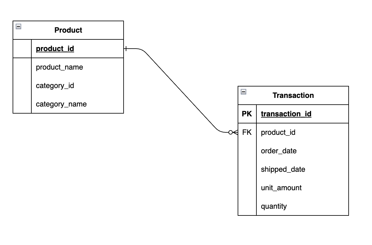
We joined Category to Product. And the grain or level of detail of Product is still at product level. And if you look at the data in this new Product table, fields from Category are repeated or redundant:

product_id,product_name,category_id,category_name
1,T-Shirts,1,Clothing
2,Dresses,1,Clothing
3,Shoes,2,Footwear
4,Smartphones,3,Electronics
5,Laptops,3,Electronics

If you’re wondering why I didn’t add “product_sk“ (surrogate key) instead, I didn’t add it in this example for the simplicity sake. I’ll be covering surrogate keys in a later section.

You could even denormalize it even further by putting everything into one table:

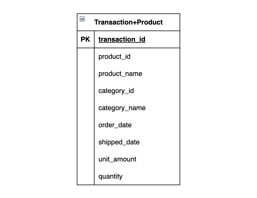
And the data in that table looks like this:

order_id,product_id,product_name,category_id,category_name,order_date,shipped_date,unit_amount,quantity
1,1,T-Shirts,1,Clothing,2025-02-01,2025-02-03,24.99,2
2,2,Dresses,1,Clothing,2025-02-02,2025-02-05,59.99,1
3,3,Shoes,2,Footwear,2025-02-03,2025-02-06,89.00,1
4,4,Smartphones,3,Electronics,2025-02-04,2025-02-07,699.00,1
5,5,Laptops,3,Electronics,2025-02-05,2025-02-08,899.00,1
6,1,T-Shirts,1,Clothing,2025-02-06,2025-02-09,24.99,3
7,3,Shoes,2,Footwear,2025-02-07,2025-02-10,89.00,2
8,6,Sandals,2,Footwear,2025-02-08,2025-02-11,45.50,1
9,7,Headphones,3,Electronics,2025-02-09,2025-02-12,129.99,2
10,8,Backpacks,4,Accessories,2025-02-10,2025-02-13,79.99,1

Values like product_id and product_name are now repeating as well as values in category related fields, because the grain of the table is now transaction.

And that’s what denormalization is all about in a nutshell. It’s crucial to understand database normalization and denormalization in order to build dimensional models.

In the next section, we’ll cover the components of a dimensional model, or a star schema.

Facts and Dimensions

Let’s cover building components of a dimensional model. It is mainly made up of 2 types of tables—fact and dimension tables. And a dimensional model is built around a business process such as sales (a customer purchasing a product), new signups (a user signing up for an app), and class attendance (a student attending class). You can identify a business process by looking for the verbs or measurable events.

Fact Table

A fact table contains facts or measures of a business process. In our earlier example, our measures would be things like unit_amount, quantity, sales_amount (unit_amount x quantity). Each row in a fact table represents a specific event at a defined level of detail, known as the grain. Fact tables also link to dimensions for the descriptive context needed to analyze those measures.

Types of Fact Tables

There are multiple fact table types to handle different business processes and to enable efficient downstream analytics and reporting.

There are mainly 3 types of fact tables:

• Transactional Fact Table: One row per event. e.g. Sales transactions

• Periodic Snapshot Fact Table: Capture the state of something at a point in time. e.g. Daily bank account balance

• Accumulating Snapshot Fact Table: Track a process with milestones. e.g. Sales order lifecycle (ordered → shipped → delivered)

While fact tables typically store numeric measures such as sales_amount and quantity, there are cases when you treat the row count of the fact table as a measure (e.g. students’ class attendance). And those tables are called Factless Fact Tables.

We will dive deeper into details of each fact table type in a future article.

Types of Measures

We store measures in fact tables, and there are a few types of measures:

• Additive Measure: Metrics that can be summed across all dimensions. e.g. Sales amount can be summed across any dimension like products, customers, and time.

• Semi-Additive Measure: Metrics that can be summed across some dimensions. e.g. Account balances can be summed by customers, branches, etc, but NOT by time.

• Non-Additive Measure: Metrics that cannot be summed across any dimension. e.g. Averages, percentages, ratios, that are typically calculated in a downstream BI/analytics tool.

We need to keep those types in mind, as they’re crucial in calculating and building accurate measures/metrics.

Dimension Table

A dimension table represents a business entity that is to slice, filter, and group facts or measures in a fact table. Dimensions help answer questions like:

• Who made the purchase?

• What product was sold?

• When did it happen?

• Where did it occur?

Fact tables store the measures of a business process, but by themselves provide little to no meaning. Dimensions provide the descriptive context needed to interpret those measures.

For example, a sales fact table may contain measures such as quantity and sales_amount, but dimensions allow them to be analyzed by different perspectives, such as:

• Date — when the sale occurred

• Customer — who made the purchase

• Product — what was sold

• Store — where the sale happened

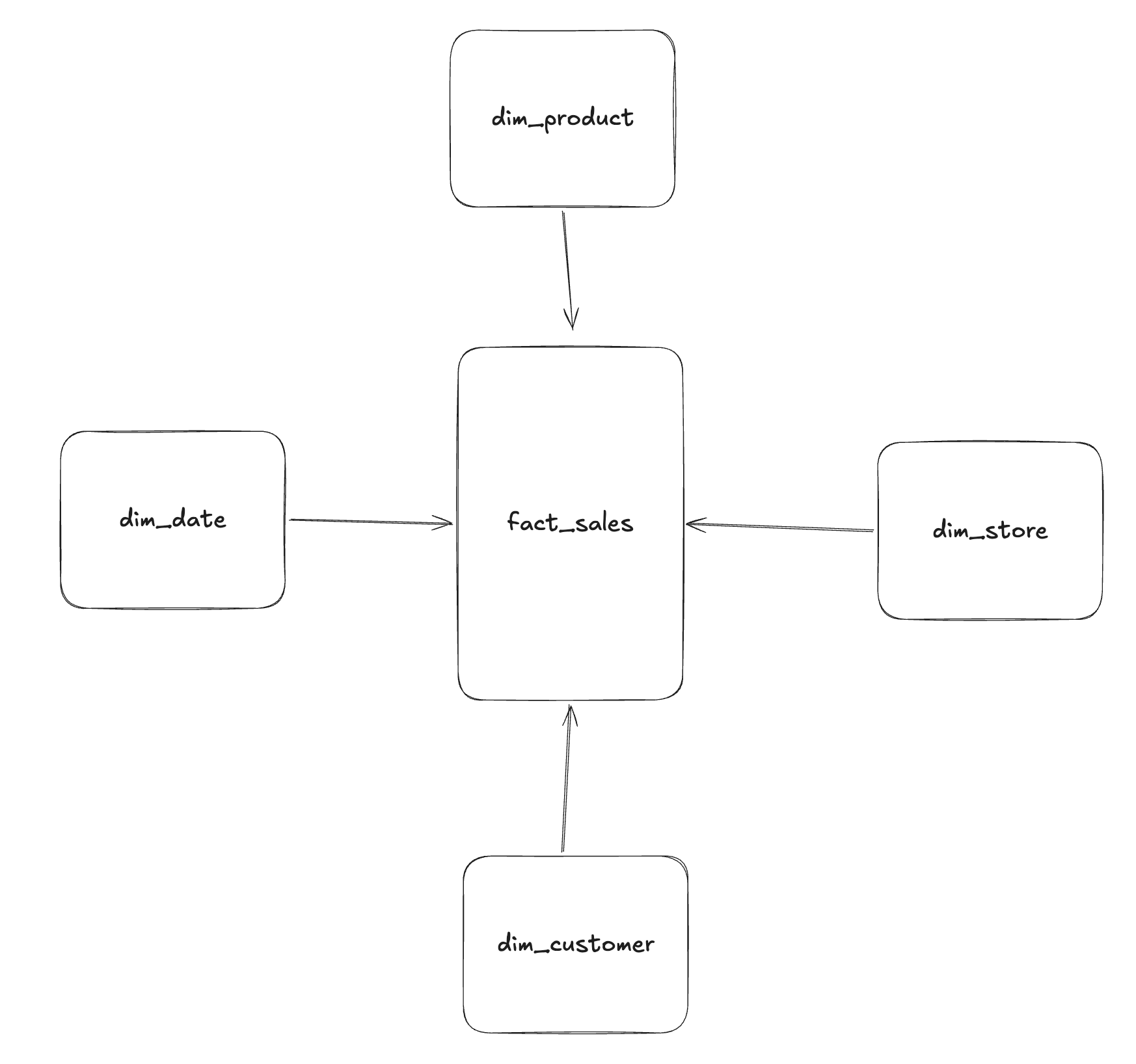
Together, fact tables and dimension tables form a star schema, where the fact table sits at the center and dimensions surround it to provide analytical context.

Dimension Attributes

Dimension tables contain attributes that describe the entities involved in a business process, such as customers, products, or dates.

Examples:

• Customer

  • customer_name

  • country

  • signup_date

  • segment

• Product

  • product_name

  • category

  • brand

• Date

  • week

  • month

  • year

• Store

  • store_name

  • store_location

Key Concepts

Dimensions key concepts:

• Conformed Dimensions: Some dimension tables are shared across multiple fact tables. This allows metrics from different processes to be analyzed together and ensures data consistency and integrity of dimension attributes.

• Slowly Changing Dimensions (SCD): Techniques used to handle changes in dimension attributes over time. e.g. A customer might move to a new city or change their name. SCD tables can track these changes to allow historical analyses.

• Surrogate Key: System-generated IDs used as the primary key in dimension tables. Instead of relying on IDs from source systems, you’d often create stable, unique keys in dimension tables so fact tables can reliably reference them, even if source system IDs change.

We’ll cover details of each dimension table type and associated concepts in a future article.

Dimensional Model Design Process

When building a dimensional model, a typical process looks like:

1. Select the business process

2. Declare the grain

3. Identify the dimensions

4. Identify the facts

This process helps you consider the business needs of the analytical model you’re trying to build, and source data availability and constraints that might exist.

It is very crucial in a successful modeling project, but is often overlooked. Make sure to start with those 4 steps in every dimensional modeling project.

Example Dimensional Model (Star Schema)

Let’s select a business process to show a concrete example in an diagram.

1. Business process = Sales transactions (customers purchasing products)

2. Grain = One row per sales transaction (or one row per order line item)

3. Dimensions = Date, Customer, Product, Store

4. Facts = Quantity, Unit Amount, Sales Amount

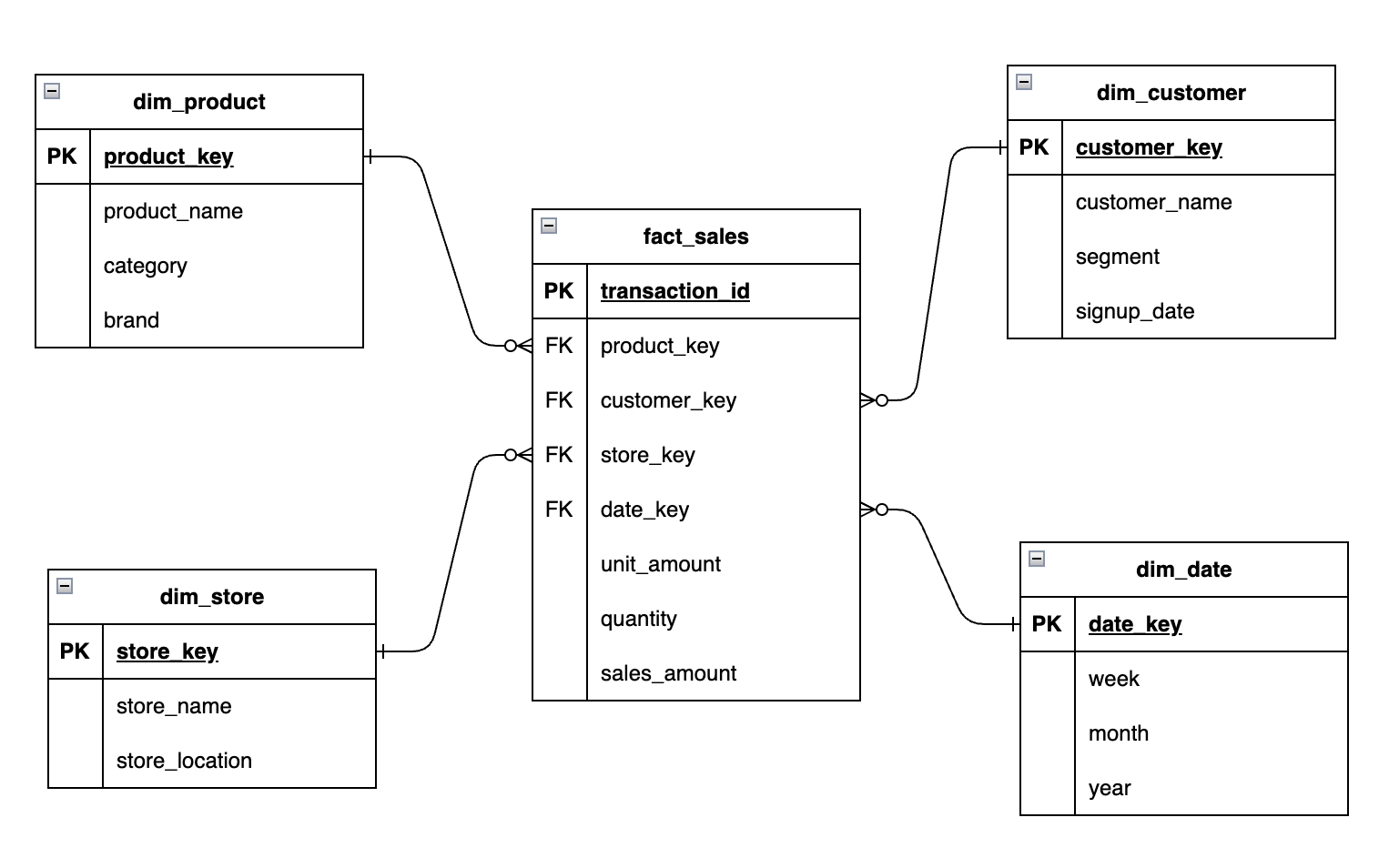
In this example, we added the surrogate key in each dimension table. You typically don’t add a surrogate key in a fact table, because the combination of foreign keys from dimension tables already creates a unique composite primary key. And, there is no functional benefit and you’d end up with the overhead of maintaining a separate, meaningless column.

When you really need a dedicated unique key for your fact table then there is usually the business key from source that you can use (e.g. transaction_id in our example above).

Other Data Modeling Techniques

Let’s compare other modeling approaches. Keep this in mind though—modeling approaches are often complementary, not mutually exclusive.

Inmon Corporate Data Factory

Inmon’s data modeling approach is often contrasted with the dimensional modeling approach popularized by Kimball, but they’re not as mutually exclusive as people sometimes make them sound.

Inmon’s approach focuses on building the enterprise-wide, trusted, integration layer in normalized data structures (3rd normal form) to act as a single source of truth. Since implementing such an architecture is time-consuming and resource-intensive, it may not make sense for many, non-enterprise companies to invest in Inmon’s approach.

In the reporting/mart layer, dimensional models can be built, taking advantage of the benefits of dimensional modeling within/on top of Inmon’s data modeling method.

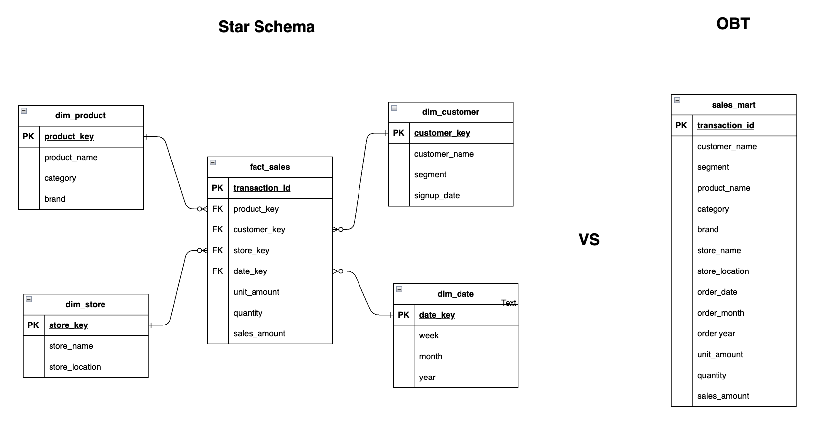
OBT (One Big Table)

As the name suggests, OBT is an approach where all relevant data is combined into a single wide table for analysis. Instead of separating facts and dimensions, everything is denormalized into one table to simplify queries and improve performance.

OBT is often used in mart tables joining fact and dimension tables so they’re reporting-ready for BI and analytics consumption.

Data Vault

Data Vault is a modeling approach for building scalable and auditable data warehouses. It separates business concepts, relationships, and descriptive context into hubs, links, and satellites. This makes it easier to integrate data and track historical changes. It typically uses an append-only approach, which supports auditability and change tracking.

Data Vault is considered more of an advanced technique that requires more experience and is more complex to query data from it compared to other techniques.

source: https://www.montecarlodata.com/blog-data-vault-architecture-data-quality/

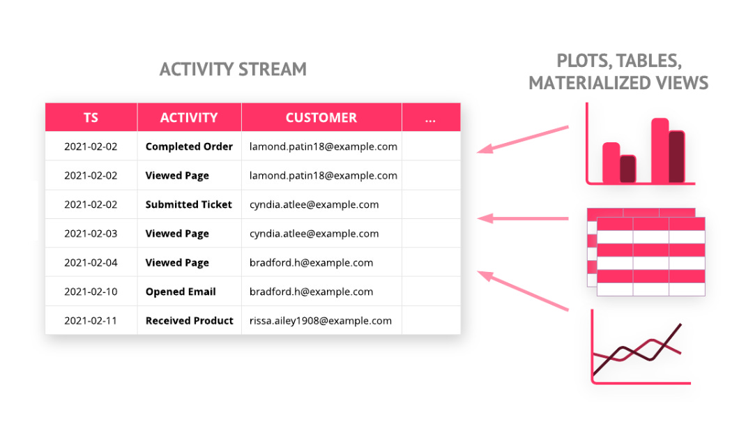
Activity Schema

Activity schemas model data around individual events or activities. It’s designed to make modeling and analysis simpler and faster by putting everything into one, time-series table.

source: https://www.activityschema.com

When Should You Use Dimensional Modeling?

You’ll need to take a step back and look at the overall picture to make the decision on your data modeling approach. And the question should be more like “Where should you use dimensional modeling in your data process?“. Maybe you don’t need it after all, but as you can see in the following diagram, dimensional modeling can often be used with other modeling approaches:

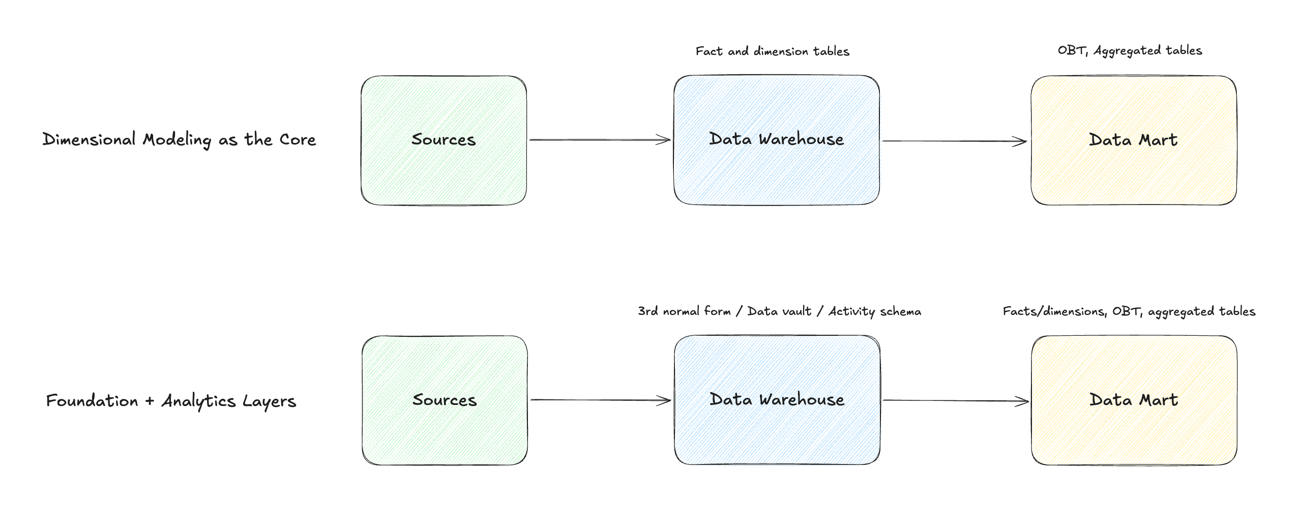
This flexibility makes dimensional modeling popular and useful across many companies and industries.

If you’re curious about why I haven’t brought up “medallion architecture“, it’s because it’s NOT a modeling approach but is just a layering or organizational pattern.

Summary

Dimensional modeling is a simple yet powerful approach to designing data for analytics. It organizes data into fact and dimension tables, balancing denormalization for query performance with principles of normalization. And, it is complementary to other modeling approaches, making it easy to integrate into a broader data architecture.

Here are some of the resources I highly recommend to learn more about dimensional modeling:

Some links below are affiliate links. If you purchase through them, it supports the newsletter at no extra cost to you. But I only recommend tools I actually use.

• Books

  • The Data Warehouse Toolkit: The Definitive Guide to Dimensional Modeling

    • Many people read this as an introductory book to dimensional modeling. It covers from the overview of dimensional modeling to specific case studies for different kinds of companies.

  • Star Schema The Complete Reference

    • This book teaches you the ins and outs of specific components of a dimensional model. You’ll have a much better understanding of exactly how to build a dimensional model after reading each chapter, and you can use the book as a reference you can always come back to when needed.

  • Agile Data Warehouse Design: Collaborative Dimensional Modeling, from Whiteboard to Star Schema

    • You’ll learn a practical, collaborative way of building dimensional models, including specific questions to ask the business to get necessary requirements for modeling.

• Websites (free)

  • Kimball Group Website

  • Data Engineering Wiki